Results
The results are structured in what was obtained for the measurements of ctobssim, ctlike and the pipeline analysis. There is a brief introduction before each of these results are presented.
The parallel parts of the monitored functions have been parallelized using OpenMP. Monitor was used to set the environment variable OMP_NUM_THREADS to different values in order to insure that the software could not access more than a specified number of cores.
In order to get the time spent in the serial and parallel parts of the programme, logging statements were added to the source code, statements which logged the duration of the parallel portion. These values were then interpreted according to Amdahl’s Law and the theoretical speedup was ploted together with the measured values.
monitor checks
Before the actual monitoring begins, a few simple test cases have been used to ee if the monitor actually does its job.
CPU usage test
The CPU usage test serves the purpose of testing if monitor can actually set the number of threads that the program is using i.e. if it correctly exports the OMP_NUM_THREADS variable correctly.
In pseudocode, the CPU test program looks like:
#pragma omp parallel
while (difftime(end,start) < interval)
        int a = 1 + 1;
This will create as many threads as the OMP_NUM_THREADS variable allows.
The results of running this through monitor are presented below.
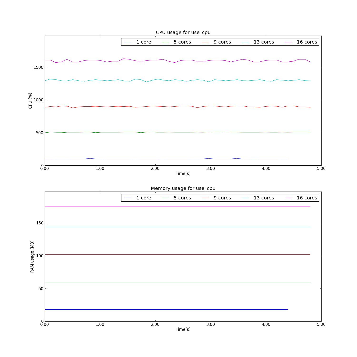
As can be seen from the plots, the CPU usage is properly monitored when there are multiple cores being employed. A somewhat strange side effect is the increase in memory as the number of cores increases.
Disk I/O
In order to test for disk I/O, a simple Python testcase was developed that simply wrote a large file to disk. In pseudocode, it would look like:
def fits_gen(file_size):
    import numpy as np
    from astropy.io import fits

    data = np.zeros(file_size * 1024 ** 2 / 8)
    fits.writeto('data.fits', data=data, clobber=True)
The chosen filesize was 5 GB. Below, you can see the results of this measurement:
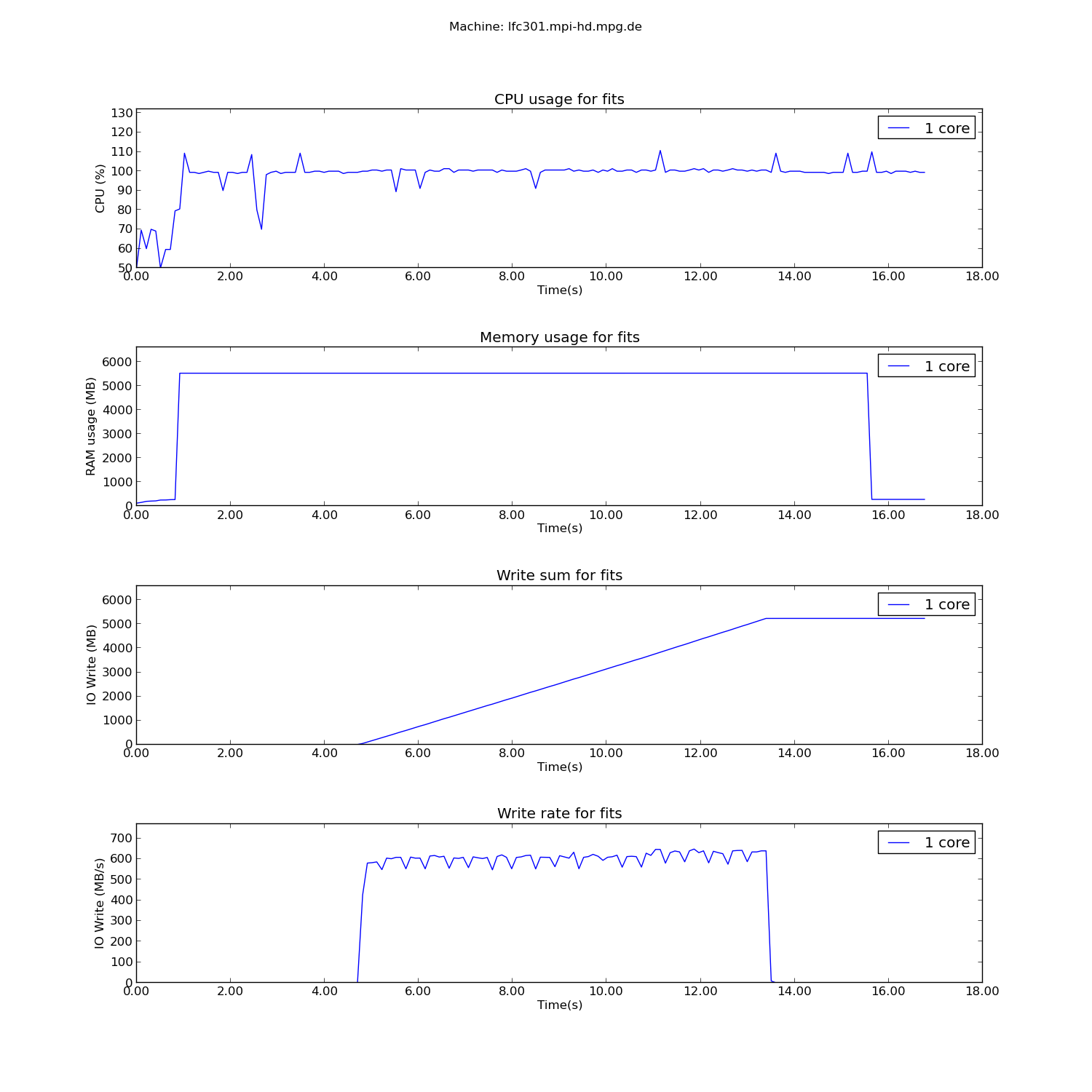
As can be seen from the plot, the cumulative write size is 5 GB and also the memory usage is about 5 GB, the extra coming from the libraries that need to be loaded. Therefore, the Monitor class and its methods yield accurate results when it comes to disk I/O.
ctobssim
Description
ctobssim is a function from the ctools suite. It is used to simulate astronomical observations given certain input parameters. For more details about the possible input parameters, see the official documentation.
The parallelism in ctobssim is realized at observation level. In short, this means that, in order to be able to see more than one CPU being used at a certain point in time, one needs to simulate more than one event. This is what we also did, as detailed in the next section.
In pseudocode, ctobssim looks like:
model = read_model("model.xml")
observations = read_observations("observations.xml")
event_lists = make_empty_lists(observations.size())

# omp parallel for
for (i = 0; i < observations.size(); i++)
    event_lists[i] = simulate_events(observation[i], model)

for (i = 0; i < observations.size(); i++)
        event_lists[i].save_to_file()
Input data
The input parameters for ctobssim were the following:
- Astronomical model Crab and Background
- Calibration database $GAMMALIB/share/caldb/cta
- Instrument response function cta_dummy_irf
- RA 83.63
- DEC 22.01
- Duration of observations 5000 s
- Energy range 0.1 - 100 TeV
- Number of simulated runs 100
Results
The results for the measurements of ctobssim are presented below.
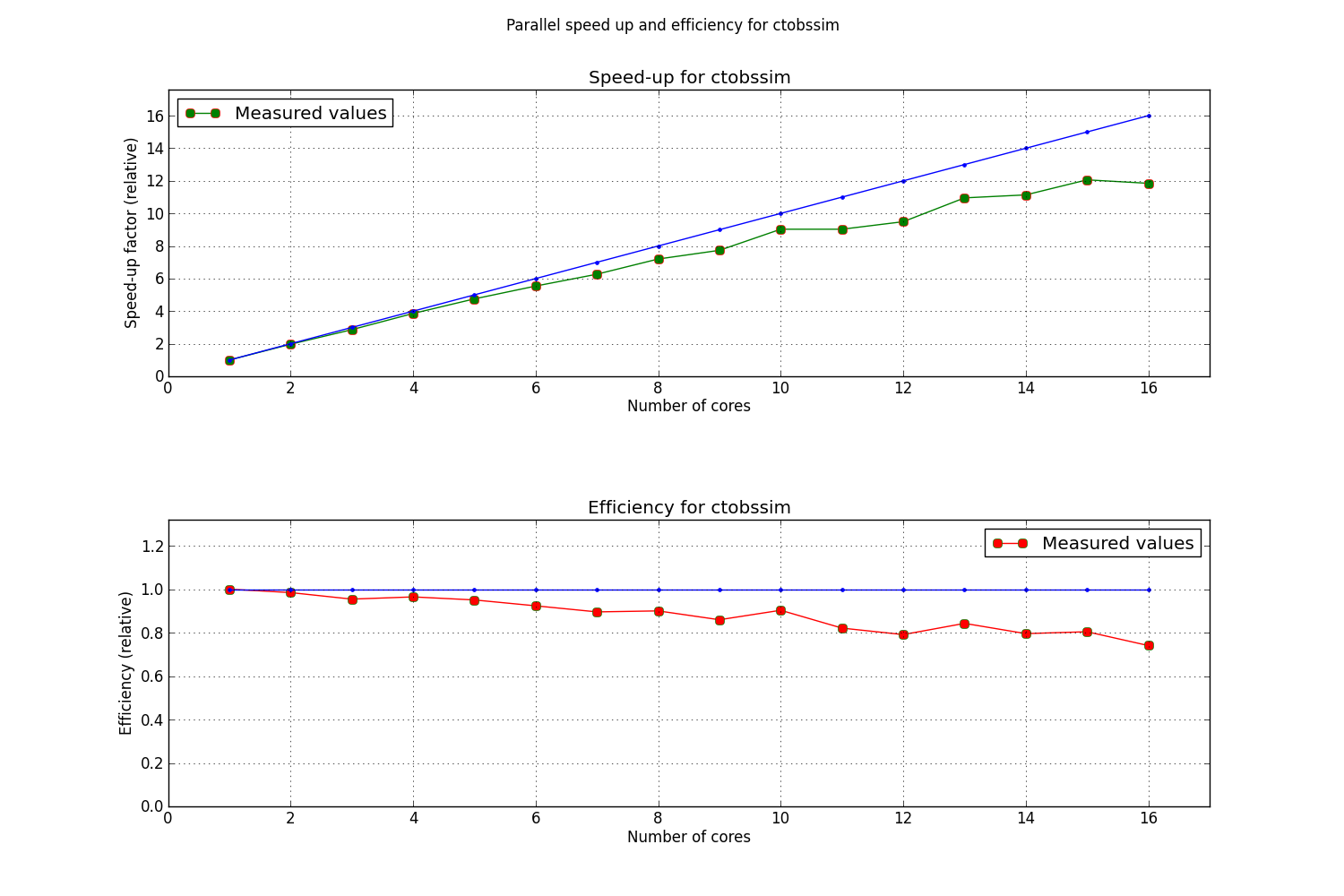
The vertical lines on the plots represent the limits of the parallel portion of the code for the execution on 1 core. This parallle_time(1) was then plugged into Amdahl’s Law in order to obtain the predicted speedup of the process.
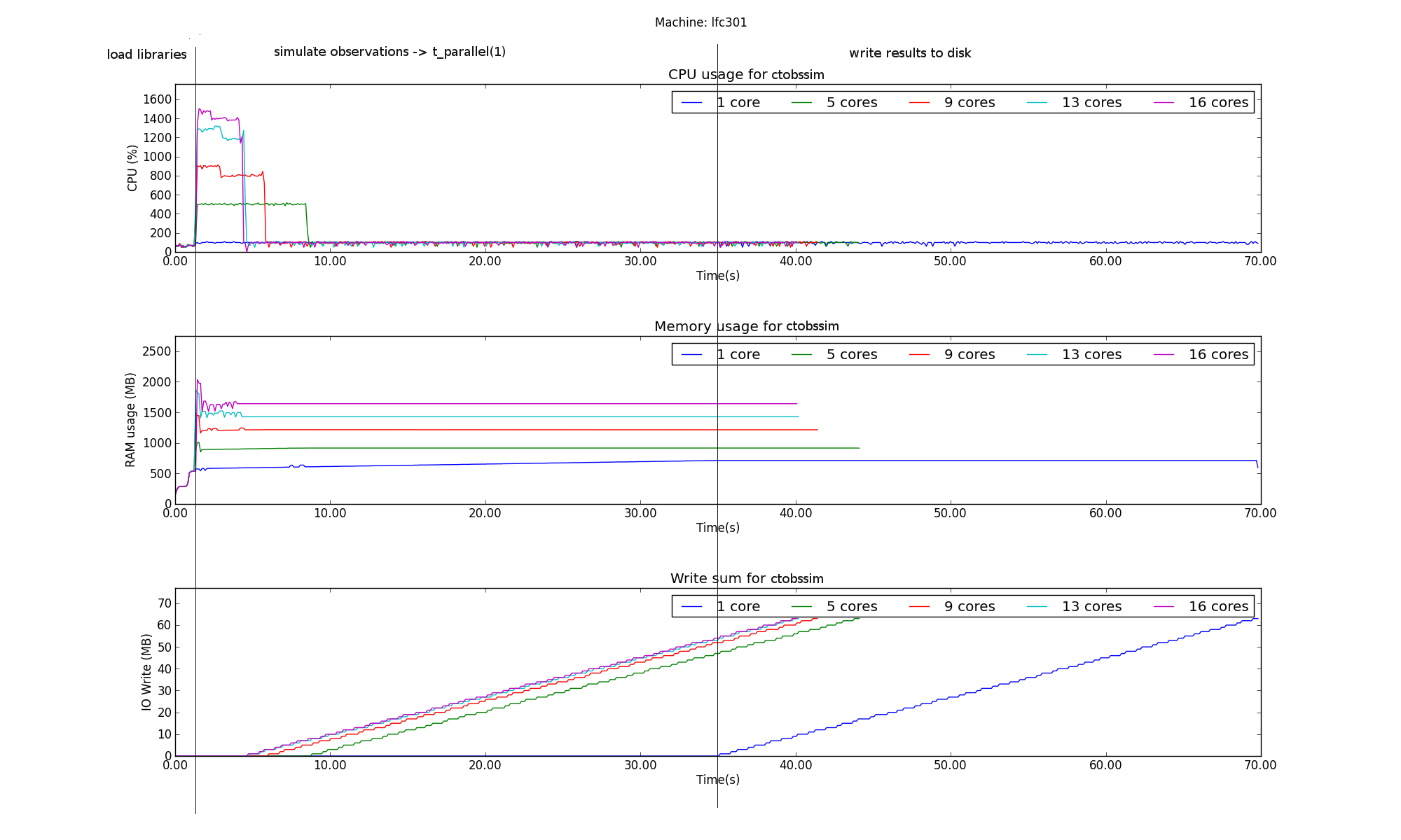
The plots show that the serial part of the program and especially the part in which I/O is done is the most time consuming one. We can therefore assume that for a process with such long serial execution time, the speedup obtained from executing the process in parallel will not scale linearly.
Below is a plot of the overall speedup of the process.
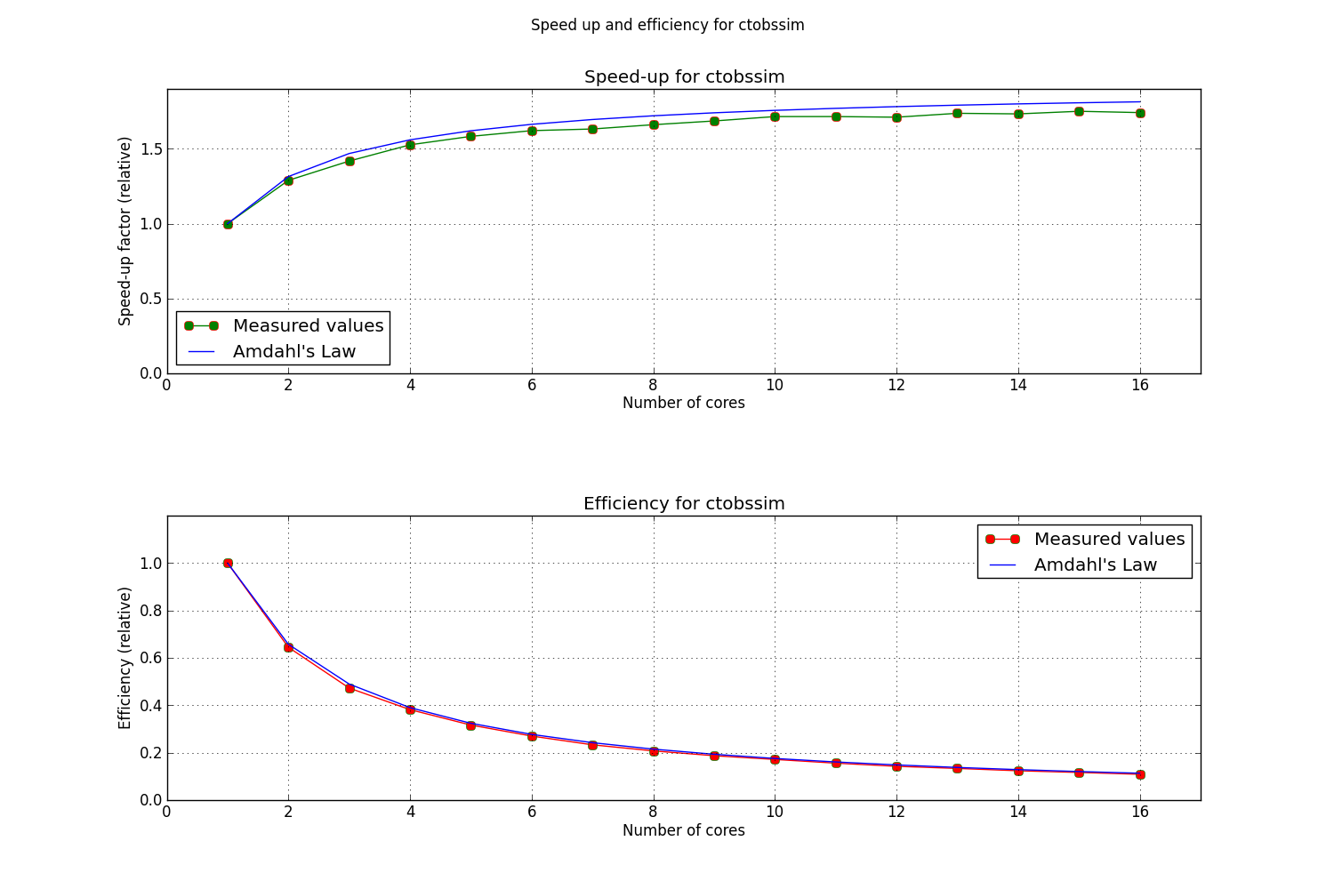
As can be seen, the execution of ctobssim respects Amdahl’s Law almost prefectly.
A closer look to how the execution time of the parallel portions of the code scales with time reveals however that there is probably some overhead that does not allow a linear scaling with time.
ctlike
Description
ctlike is another function from the ctools suite. It takes as input parameters a list of observations and it computes the maximum likelihood fit for that list of parameters. For more details about the possible input parameters, see the official ctlike
The parallelism in ctlike is implemented again at observation level.
In pseudocode, ctlike looks like:
model = read_model("model.xml")
observations = read_observations("observations.xml")
data = read_data("data.xml")
optimizer = make_optimizer(model, observations, data)
optimizer.run()
optimizer.model.save_to_file("fitted_model.xml")
void Optimizer::run(){
        // détails not important here …
        // calls compute_likelihood() in a while loop
        // typically 100 to 1000 times until convergence is achieved
        while (..)
                this->guess_new_model_parameters()
                this->compute_likelihood()
}

void Optimizer::compute_likelihood(){
        likelihoods = std::vector<double>(this->observations.size())
        # omp parallel for
        for (i = 0; i < observations.size(); i++)
                // The per-observation likelihood is an expensive computation that
                // could be further parallelized … but details are not important here
                likelihoods[i] = compute_likelihood_for_one_observation(i)
        self->likelihood = likelihoods.sum()
}
Input data
- Astronomical model Crab and Background
- Source of data ctobssim simulated runs
- Events/run 360
- Analysis type unbinned
- Energy range 0.1 - 100 TeV
- Number of evaluated runs 100
Results
The results for ctline are presented below.
As can be seen, even though ctlike is allowed to use for example 16 cores, it will only 14 or 15 cores for the simulation. This behaviour has not yet been properly explained.
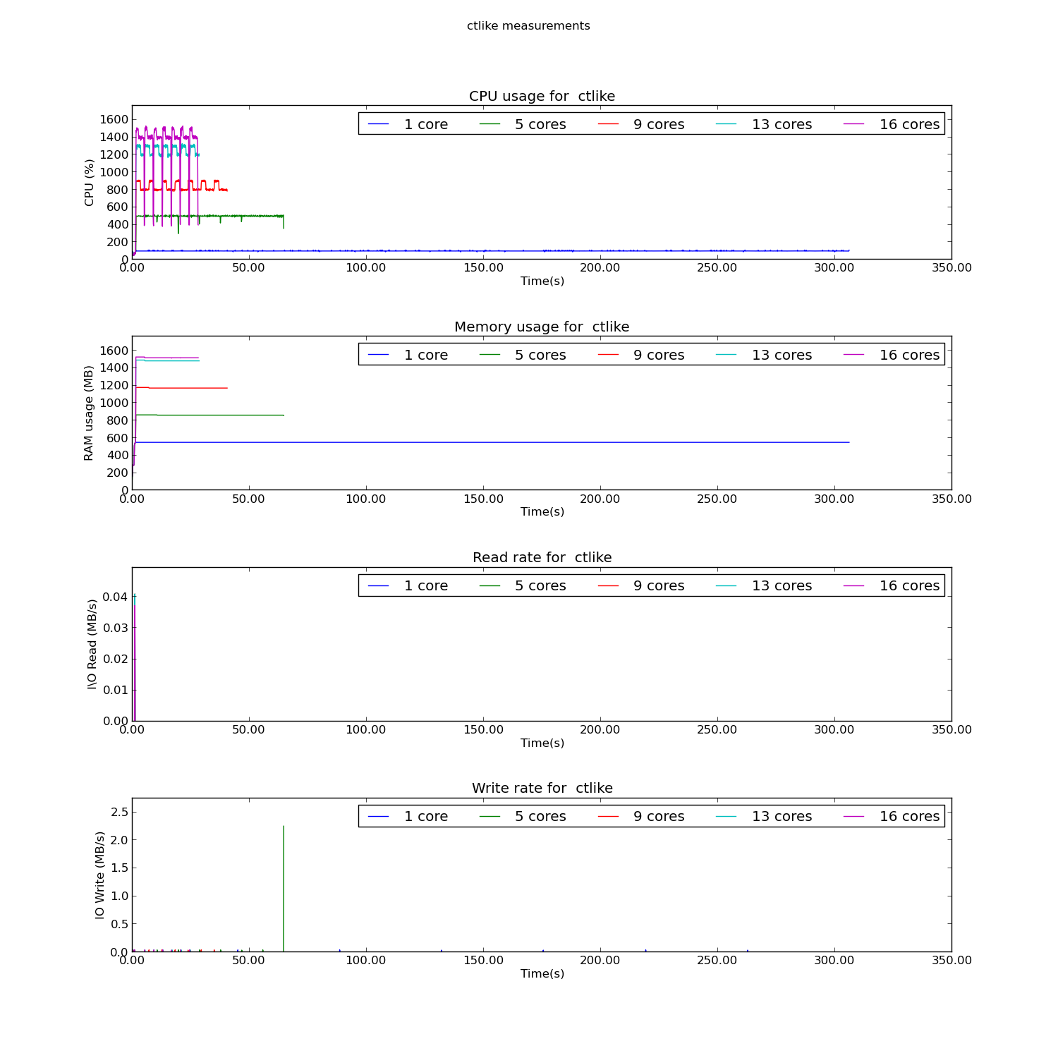
As was expected, ctlike is doing almost no I/O at all. Another important point to note is that the biggest part of ctlike is parallelized so we can expect good speedups when using multiple cores.
The measured speedup does not conform with the value predicted by Amdahl’s Law. However, it can be seen that the execution time is greatly reduced when using multiple cores. Further investigation is needed to see why the OpenMP parallelization fails to yield an ideal efficiency.
pipeline analysis
Description
The pipeline analysis consists of different that are run consecutively. Thus, the events are simulated by ctobssim, they are filled into enegy bins using ctbin and the maximum likelihood fit is computed using ctlike.
The advantage of the pipeline is that it can run these events one after the other instead of separating the processes from one another. Another advantage is that the data can be stored in memory thus relinquishing the need to physically save the results to disk.
As before, parallel behaviour can be observed only when running the pipeline for more than one event. The parallelized portions of the code lie in ctobssim and ctlike while ctbin contains only serial code.
Input data
The pipeline was run with the following input data:
- Astronomical model Crab and Background
- Calibration database $GAMMALIB/share/caldb/cta
- Instrument response function cta_dummy_irf
- Duration of observations 5000 s
- Energy range 0.1 - 100 TeV
- Number of simulated runs 100
Results
The results of the in memory pipeline can be seen below.
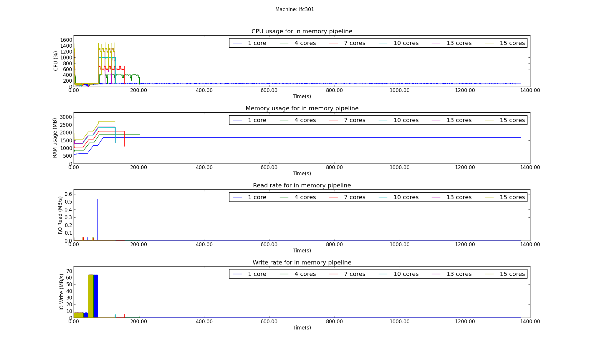
As can be seen, the execution on a single core takes a lot more time than it does on multiple cores. This has a strong effect on the efficiency as can be seen in the next plot.
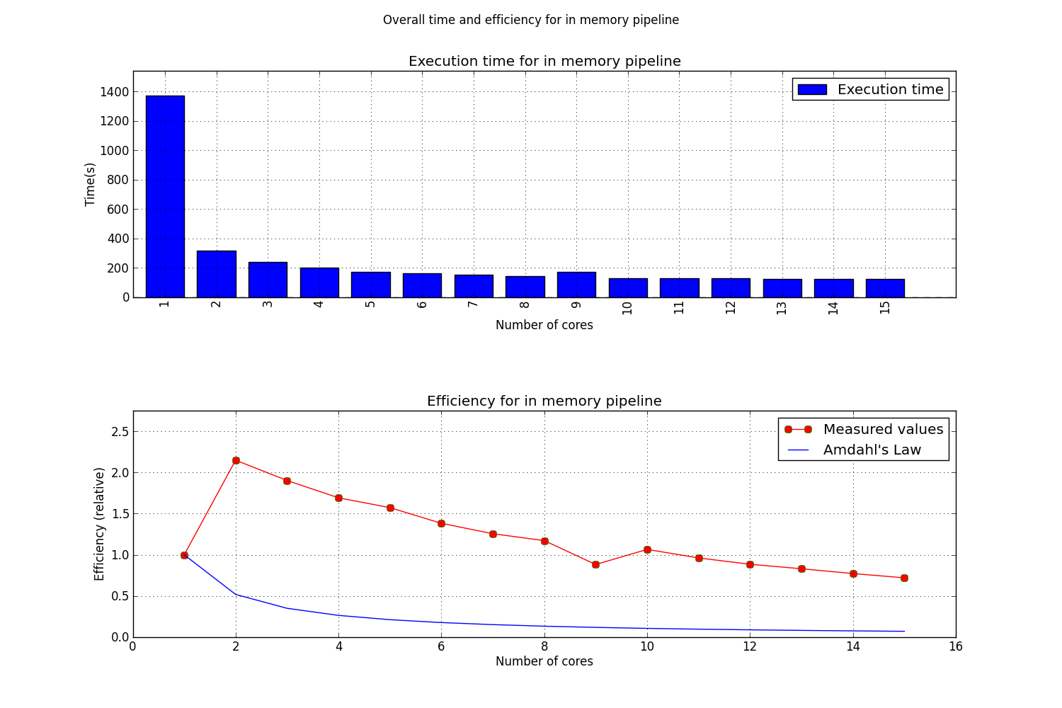
The multiple core execution time is much shorter than the single core time. This will lead to a measured efficiency greater than 1! It was not yet determined why this happens. Even though the pipeline analysis was run multiple times, it yielded similar results each time.